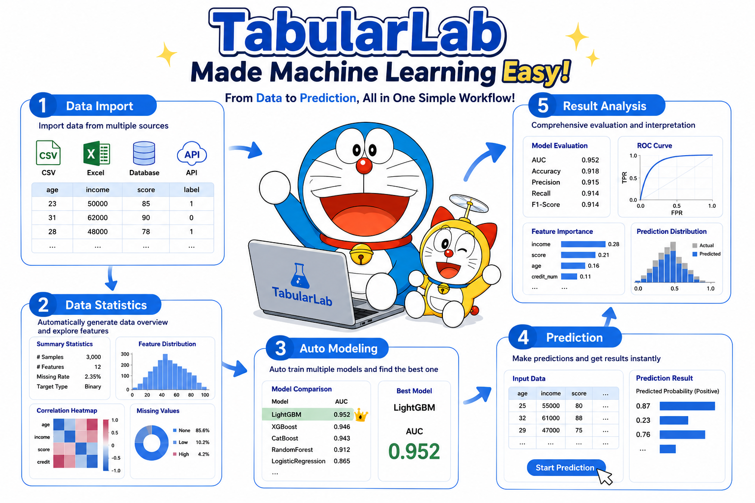
This manual is written for beginners. You do not need to write code. Prepare a spreadsheet, then follow the workflow: import data, choose a task, define column roles, train a model, read results, export figures, and make predictions.
TabularLab processes your table locally in the browser or desktop app. It is suitable for teaching, early-stage research analysis, material data exploration, small tabular ML projects, and publication-ready chart export.
2. Quick Start: run one analysis in about five minutes
If you do not have your own data yet, start with a built-in sample dataset.
Download the software
Download a desktop app from the release page, or open index.html in a browser.
Load sample data
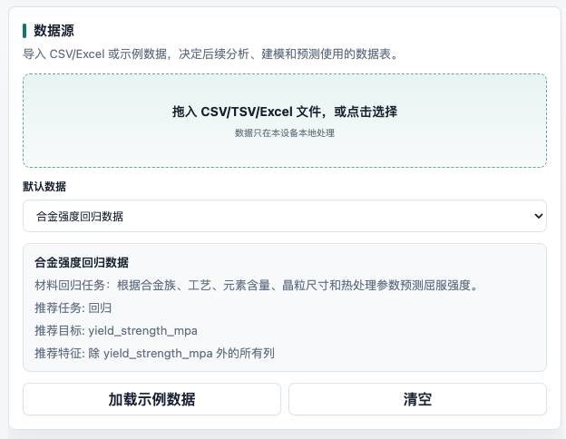
Choose a default dataset in the Data Source panel and click Load Sample.
Check the task
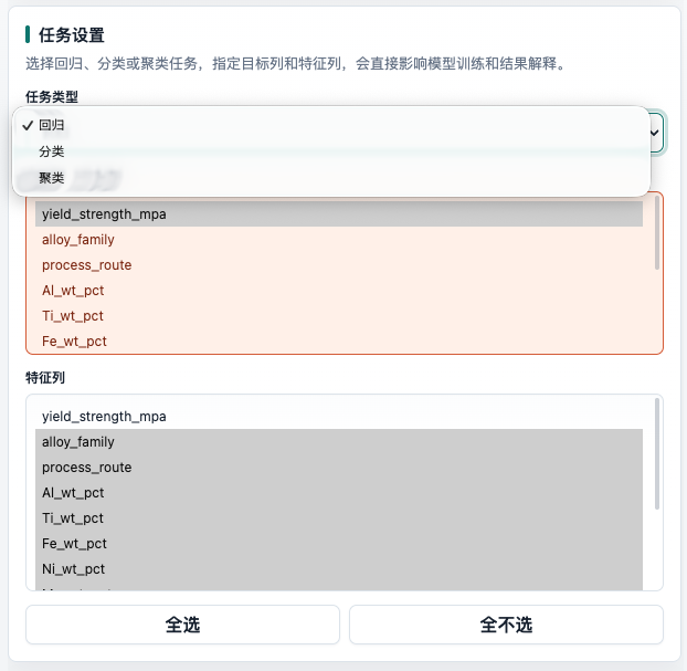
Confirm the task type, target columns, and feature columns in Task Setup.
Train the model
Choose preprocessing and model settings, then click Run Analysis.
Read results
Open the Results tab to inspect metrics, summary report, and result plots.
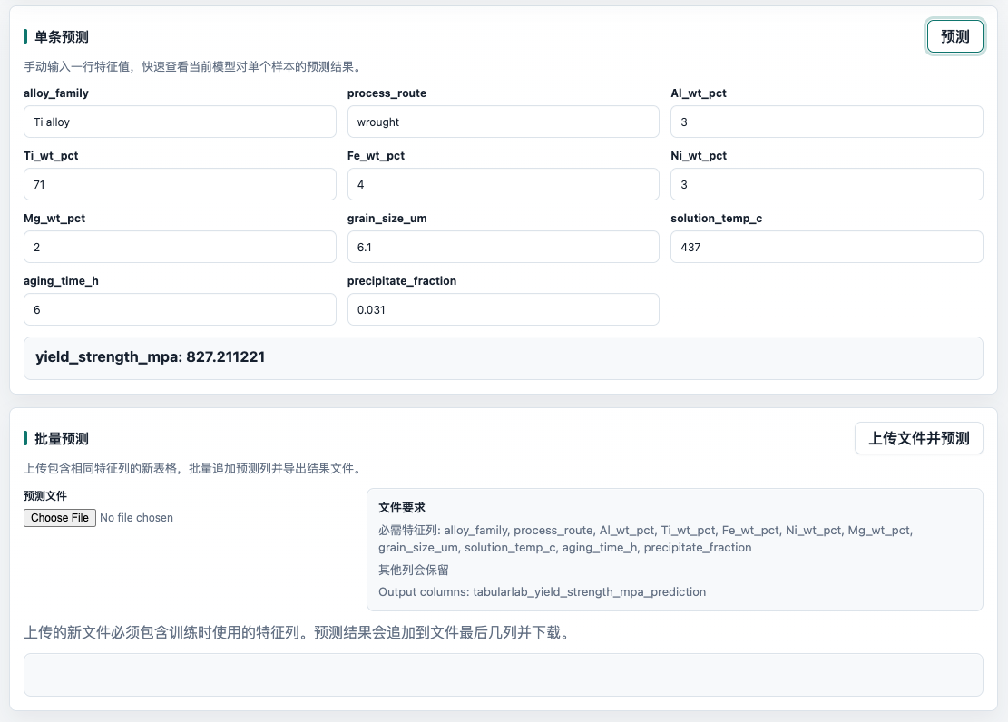
Predict new data
Use the Predict tab for single-row prediction or batch prediction from a file.
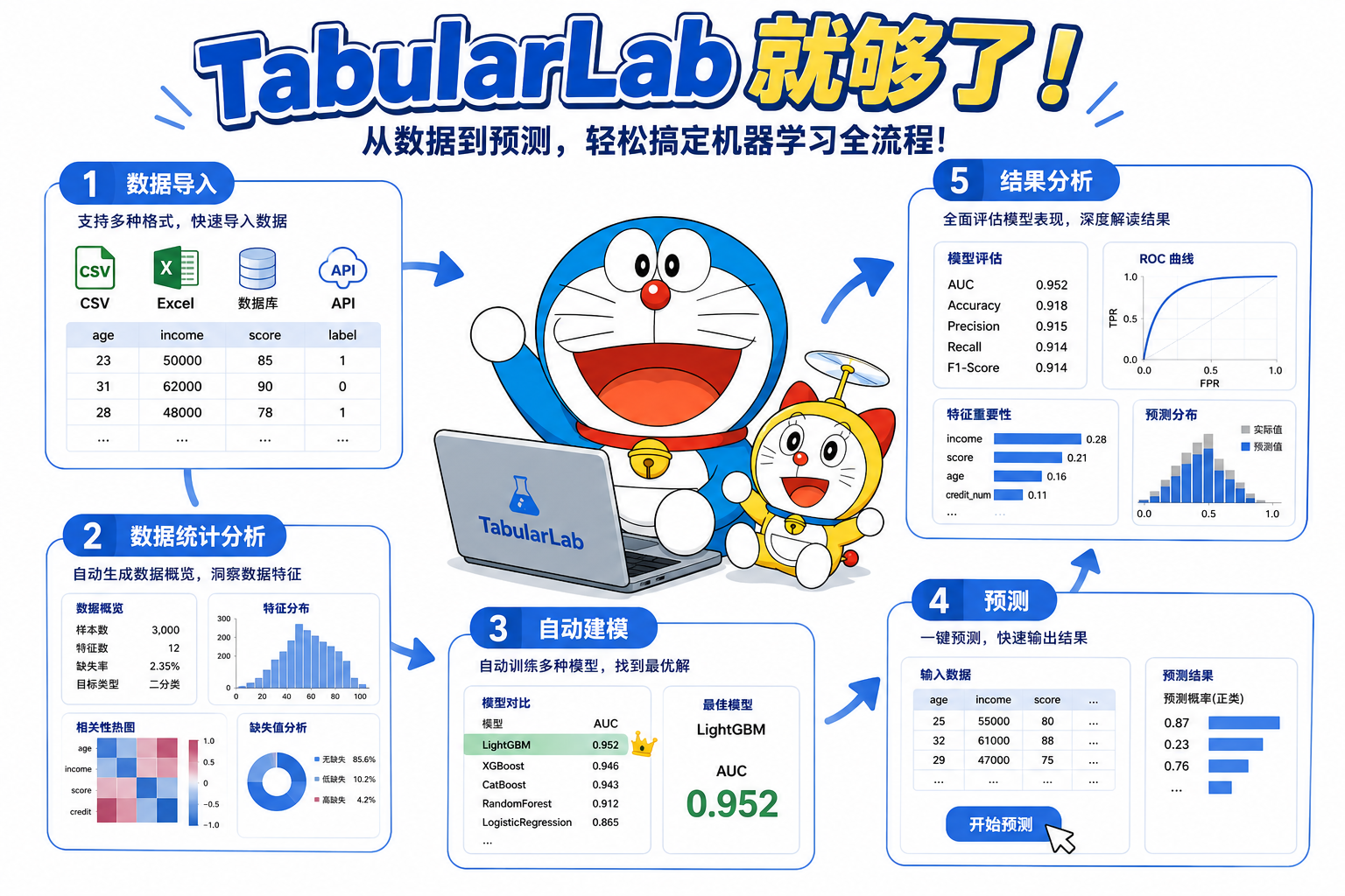
Figure 1: Load a sample dataset. Beginners should first run a sample before using their own table.
Appendix: Machine Learning Basics for Beginners
Machine learning means learning a relationship from existing examples, then applying that relationship to new samples. In TabularLab, the examples are rows in a table, and the information used by the model is stored in columns.
Sample / row
One row is one sample, such as one material, experiment record, student, or product. The model learns from many rows.
Variable / column
One column is one type of information, such as density, temperature, process route, class label, or strength.
Feature column
A feature is an input used by the model, such as composition, treatment temperature, grain size, material family, or process route.
Target column
The target is the answer you want to predict. Regression and classification need target columns; clustering does not.
Training
Training adjusts a model so its predictions match known answers. The goal is not memorization, but a pattern that works on new data.
Prediction
Prediction applies a trained model to a new sample. The new table must contain the same feature columns used during training.
Train/test split
Training rows fit the model. Test rows are hidden during training and used to estimate performance on unseen data.
Cross validation
K-fold cross validation repeatedly trains on K-1 folds and validates on the held-out fold. TabularLab reports OOF predictions by combining all held-out predictions.
Regression
Regression predicts a continuous number, such as strength, capacity, price, or temperature. Common metrics include R2, RMSE, and MAE.
Classification
Classification predicts a category, such as material class, pass/fail, or low/medium/high. Common outputs include accuracy, F1, and a confusion matrix.
Clustering
Clustering groups samples without known answers. It is useful for exploration, family discovery, and anomaly inspection.
Overfitting
Overfitting means a model fits training details or noise too closely, so it looks good on training data but performs poorly on new data.
Main algorithms used by TabularLab
Algorithm
Task
Plain-language idea
Good starting point when
Linear / Ridge / Lasso / ElasticNet
Regression
Combine features with weights to predict a number.
You want a fast, interpretable baseline.
Linear SVR / Linear SVM
Regression / Classification
Find a stable linear boundary or linear prediction rule.
You have many features and roughly linear behavior.
Decision Tree
Regression / Classification
Ask a sequence of if/then questions about feature values.
You want an interpretable model, while watching for overfitting.
Random Forest
Regression / Classification
Train many trees and average or vote their outputs.
You need a robust general-purpose tabular model.
Gradient Boosting
Regression
Build models sequentially, each one correcting earlier errors.
You need stronger fitting power and can tune parameters.
KNN
Regression / Classification
Find the K most similar samples and use their answers.
Your dataset is small and similar samples should have similar results.
Softmax Logistic
Classification
Estimate class probabilities and choose the most likely class.
You need a fast multiclass baseline.
Gaussian Naive Bayes
Classification
Estimate feature distributions for each class and pick the most likely class.
You need a very fast classification baseline.
KMeans
Clustering
Split samples into K groups around cluster centers.
You roughly know the number of groups.
DBSCAN
Clustering
Build clusters from dense regions and mark isolated points as noise.
You want anomaly detection or irregular cluster shapes.
Agglomerative
Clustering
Start with one group per sample, then merge nearby groups step by step.
You want hierarchical grouping behavior.
Beginner checklist
Decide whether you need to predict a number, predict a class, or discover groups.
Make sure answer-like columns are not selected as features.
Run a default model first, then compare a small number of alternatives.
Trust test-set or cross-validation results more than training impressions.
If metrics are poor, check data quality, target choice, features, and missing values before switching to a complex model.
Do not use IDs as features unless they carry meaning
Sample IDs, random IDs, and experiment numbers usually do not describe real patterns. Using them as features can make the model learn meaningless shortcuts.
3. Full workflow
Prepare a clean table in CSV, TSV, TXT, XLSX, or XLS format.
Import the table or load a built-in sample dataset.
Choose regression, classification, or clustering.
Assign each column as feature, target, or ignored.
Set missing-value handling and categorical encoding.
Choose a model and validation settings.
Run the analysis.
Read the summary, metrics, plots, and logs.
Export charts, results, predictions, or processed data.
Use the trained model for new single-row or batch prediction.
4. Data Source: import your own table or sample data
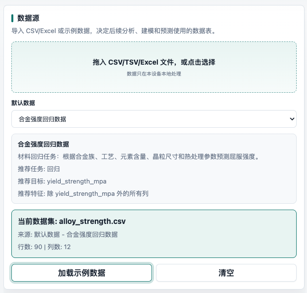
Figure 2: Data Source panel. This panel decides which table is used for the analysis.
Supported file types
.csv: recommended for most users.
.tsv / .txt: useful for tab-separated or plain text tables.
.xlsx / .xls: Excel files; TabularLab reads the first worksheet.
Import your own data
Click the dashed upload box or drag your file into it.
After import, check the current dataset name, row count, and column count.
Open Overview to inspect column types, missing values, and examples.
Data quality check
The Overview tab automatically checks high-missing columns, constant columns, ID-like or unique text columns, duplicate rows, numeric outliers, and possible target-leakage columns whose names are too similar to target names. These warnings do not delete data; they help you decide which columns need to be ignored, corrected, or reviewed.
Fix data before trusting metrics
If data quality warnings show target leakage, duplicate rows, or severe missingness, review column roles and raw data before training. Otherwise metrics may look strong while real prediction remains unreliable.
Table preparation tips
The first row should contain column names. Avoid merged cells. Each column should have one meaning. Empty cells are allowed and can be handled later by preprocessing.
The target is the answer you want to predict. Features are the input columns used to make that prediction. For clustering, there is no target column.
6. Column Roles: feature, target, or ignored
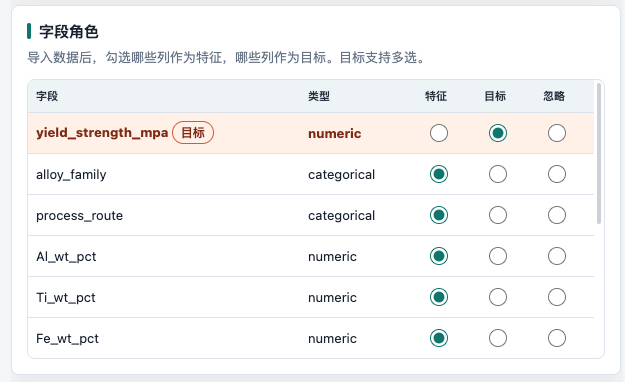
Figure 4: Column Roles table. Each column should have exactly one role.
Feature: input information used by the model.
Target: the answer to predict. Regression/classification use targets; clustering does not.
Ignore: columns excluded from modeling, such as notes, IDs, or duplicate information.
Column roles directly affect model validity
If you accidentally use an answer-like column as a feature, the model can appear very accurate but will not be meaningful.
7. Processing & Training: clean data and train a model
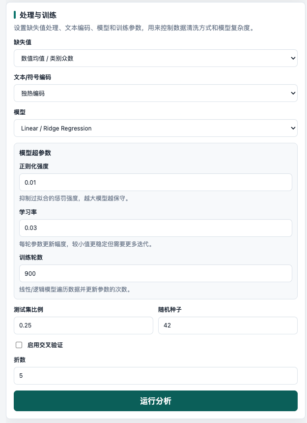
Figure 5: Processing & Training panel. Configure missing values, encoding, model, and validation settings.
Missing-value handling
Numeric mean / category mode: a good default for many datasets.
Numeric median / category mode: more robust when numeric columns contain outliers.
0 / Unknown: useful when zero or Unknown has a clear meaning.
Categorical encoding
One-hot: converts categories into separate 0/1 columns. Recommended for most categorical features.
Ordinal: maps categories to numbers. It uses fewer columns but may introduce artificial order.
Model choice
Regression: start with Linear/Ridge, Random Forest, or Gradient Boosting.
Classification: start with Softmax, Random Forest, or Gaussian Naive Bayes.
Clustering: start with KMeans; try DBSCAN for irregular clusters.
Use train/test split for a simple evaluation. Use cross-validation OOF evaluation when you want a more stable estimate across all usable rows.
Auto tuning
Auto tuning tests multiple important model-parameter settings before the final run, such as regularization strength, learning rate, tree depth, tree count, K value, or boosting rounds. TabularLab compares candidate settings with an internal validation score, writes the best parameters back into the current parameter inputs, and then trains the final model with those settings.
Bayesian tuning: a faster search over key parameters with fewer candidate trials.
Grid search: a more regular sweep over preset parameter combinations, but it can take longer.
Recommendation: run the default model first. Enable auto tuning only after the workflow is correct and you want to improve metrics. Larger datasets and more complex models will take longer.
8. Results: read more than one number
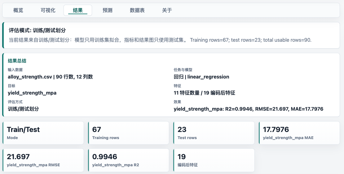
Figure 6: Results tab. It contains evaluation mode, summary report, metric cards, logs, and result plots.
Result summary
V1.1.0 adds an automatic result summary: input data, task, target, feature count, evaluation mode, and main effect metrics. It is useful for lab notes and report drafts.
Regression metrics
R2: closer to 1 is better. Negative values indicate poor performance.
RMSE: lower is better and penalizes large errors strongly.
MAE: lower is better and is easy to interpret as average absolute error.
Classification metrics
Accuracy: overall correct prediction rate.
Precision: when the model predicts a class, how often it is correct.
Recall: when a sample truly belongs to a class, how often the model finds it.
F1: a balance between precision and recall.
Clustering outputs
Cluster sizes: how many rows belong to each cluster.
Noise: DBSCAN samples not assigned to any cluster.
Projection plot: PCA, t-SNE, numeric-feature, or encoded-feature projection.
Inverse recommendation (regression only)
After training a regression model, the Results tab shows an Inverse Design panel. Enter one or more desired target performance values and choose the recommendation count Top N. TabularLab generates 30000 uniformly distributed candidate points inside the trained feature space, excludes feature combinations already present in the uploaded data, and predicts every remaining candidate with the current model.
Recommendations are sorted by the L2 distance between predicted target values and desired target values. Smaller distance means the candidate is closer to the requested performance. The report includes the search method, feature-space coverage, skipped known points, recommended feature combinations, predicted values, and errors.
Inverse constraints and export
Inverse design supports optional search constraints. Numeric features can use narrower minimum and maximum values. Categorical features can use comma-separated allowed categories. Empty constraint fields use the full imported range or all observed categories. Inverse results can be exported as CSV or JSON with Top N recommendations, L2 distance, recommended features, predicted values, errors, and search-space information.
Inverse recommendation is not an experimental guarantee
The recommendations are model predictions inside the imported feature ranges. Use them as candidate designs or experiment-priority suggestions. If the training data are sparse, metrics are weak, or key physical features are missing, the recommended points may be unreliable.
Feature importance
The Results tab shows both a feature-importance table and a horizontal bar chart. Linear models use coefficient magnitude, tree models use split counts, and other models use approximate permutation importance. The chart shows the top 20 features, while the table lists more features, importance values, and the calculation method. Use it to understand what the model relies on and to spot possible ID, leakage, or meaningless features.
9. Charts and export
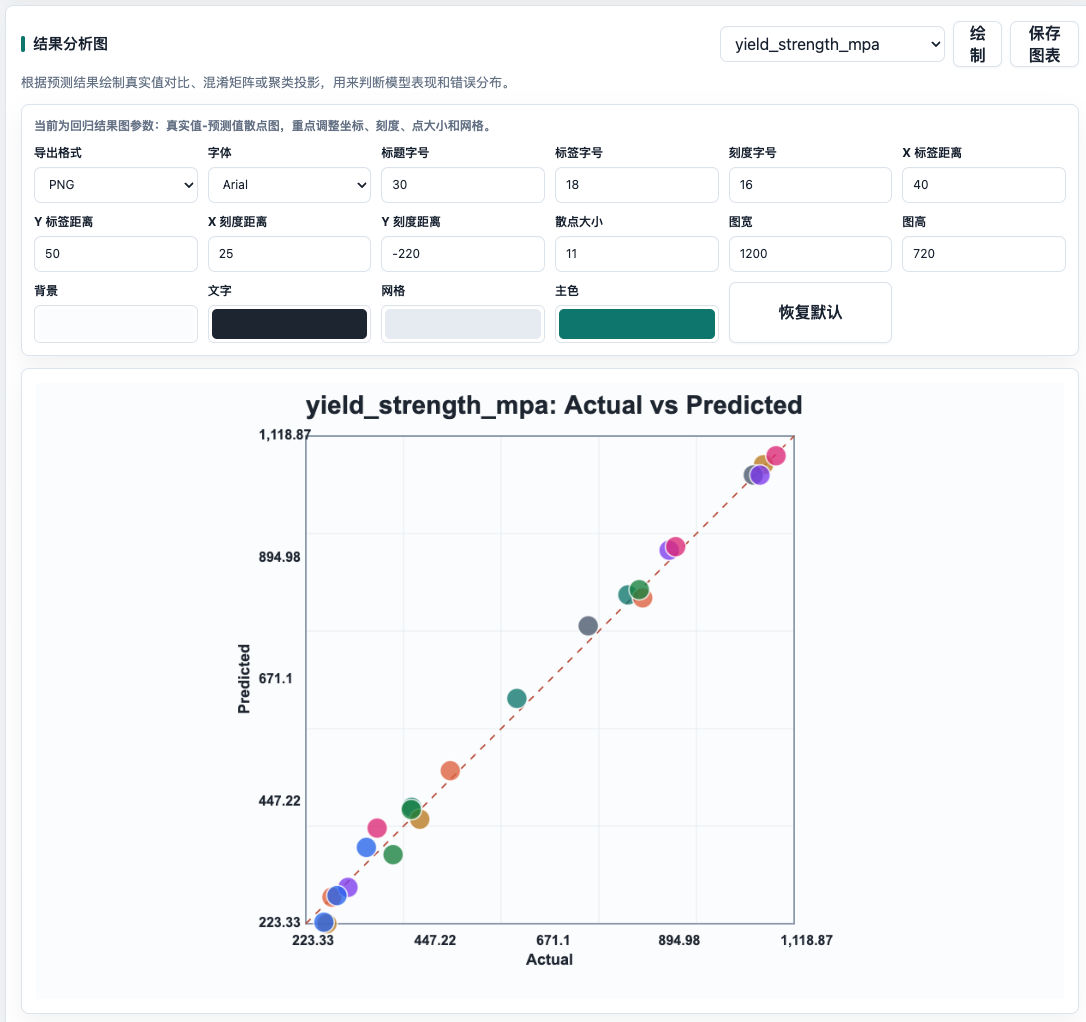
Figure 7: Result analysis plot. Different tasks show different plots and parameter controls.
Visualization tab charts
Histogram: distribution of one numeric column. Y is fixed to Count.
Violin plot: smoothed distribution shape of one numeric column. Y is fixed to Count.
Scatter plot: relationship between two numeric columns, optionally colored by target.
Correlation heatmap: correlations among numeric features; max features and color style are adjustable.
Target plot: target relationship plot for classification or regression tasks.
Result plot by task
Regression: actual-vs-predicted scatter plot.
Classification: confusion matrix with adjustable label angles, heatmap style, number size, and number color.
Clustering: projection scatter plot with PCA, t-SNE, numeric-feature, and encoded-feature projection options.
PNG or SVG
Use PNG for quick reports and slides. Use SVG for papers because it is a vector format and remains sharp when resized.
10. Prediction
Figure 8: Predict tab. Use one manually entered sample or upload a batch file.
Single prediction
Train a model first.
Open the Predict tab.
Fill each feature value for the new sample.
Click Predict and read the output.
Batch prediction
Prepare a new CSV or Excel file.
Make sure it contains the same feature columns used during training.
Upload the file and check the requirement panel.
Download the file with appended prediction columns.
Save and load models
After training, use Save Model in the Results tab to export a model JSON file. It contains the task, targets, feature columns, preprocessor, encoding information, model parameters, and trained model. Later, load that model file to continue single-row or batch prediction without retraining. A loaded model still requires new prediction files to contain the same feature column names used during training.
11. Data Preview and processed data
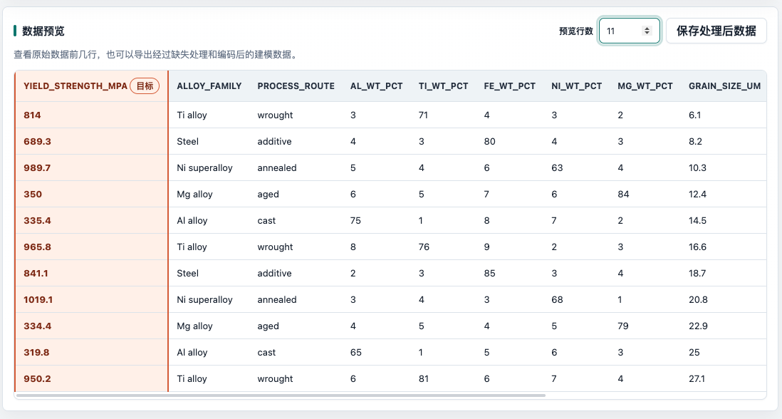
Figure 9: Preview tab. Check whether the imported data was read correctly.
Adjust preview row count to inspect more rows.
Target columns are highlighted to help verify roles.
Save Processed Data exports the modeling table after missing-value handling and encoding.
12. Export and citation
Charts: PNG or SVG.
Results: JSON with task, targets, features, metrics, and validation information.
Predictions: CSV with actual/predicted values or cluster labels.
Model: JSON with preprocessor, model parameters, and trained model, reloadable for prediction.
Inverse design: CSV or JSON with Top N recommendations, predicted values, errors, L2 distance, and search space.
HTML report: a report containing summary, reproducibility information, feature importance, inverse recommendations, and model output.
Processed data: CSV after preprocessing.
Citation: plain text citation and BibTeX.
Reproducibility information
Results JSON, HTML reports, and model output logs include reproducibility information such as software version, generation time, dataset name, task, targets, features, missing-value strategy, encoding strategy, model parameters, random seed, test size, evaluation mode, and train/test split. Save this information with exported models or result files for papers and project records.
Bin Cao. (2026). TabularLab : A lightweight toolkit for tabular machine learning. Version 1.1.0. https://github.com/bin-cao/TabularLab
13. FAQ
Why does Run Analysis not work?
Make sure a dataset is loaded.
For regression/classification, make sure a target column is selected.
Make sure at least one feature column is selected.
For regression, the target column must be numeric.
Why are metrics good but the model is not useful?
You may have included answer-like columns as features. Recheck Column Roles and remove leaked information.
Why do chart labels overlap?
Increase chart width or height, reduce font size, adjust X/Y label distance, or change X/Y label angle. For correlation heatmaps, reduce the maximum feature count.
When should I avoid using TabularLab?
TabularLab is designed for small to medium datasets, teaching, and fast exploration. It is not a replacement for validated production ML workflows in high-risk medical, financial, legal, or safety decisions.